Oracle

How to install Oracle :

·         Sql (structured query language) is for accessing databases.

·         SQL is a standard language for accessing and manipulating databases like MySQL, SQL Server, Access, Oracle, Sybase, DB2, and other database systems.

What is data?

A database is a collection of information that is organized so that it can easily be accessed, managed, and updated. Data is raw, unprocessed information. In and of itself it may not mean much.

What is information?

                Information, on the other hand, is processed data that has meaning.

What is metadata?

                Meta data is “data about data”. An item of metadata describes the specific characteristics about an individual data item. In databases, metadata describes the structural components of tables and their elements. For example, metadata about an element includes its data type, name of data, size and many more characteristics about that element. It would also give information about the tables the database is storing, information, such as length of fields, number of columns. One of the main uses of Meta data is to provide a link between the information creator and the information users.

What is database?

                A collection of information organized in such a way that a computer program can quickly select desired pieces of data. 

Traditional databases are organized by fields, records and tables. A field is a single piece of information; a record is one complete set of fields; and a file is a collection of records. For example, a telephone book is analogous to a file. It contains a list of records, each of which consists of three fields: name, address, and telephone number.

What is DBMS?

                A database management system (DBMS) is the software that allows a computer to perform database functions of storing, retrieving, adding, deleting and modifying data. In other words it is general-purpose software that provides the users with the processes of defining, constructing and manipulating the database for various applications.

History:

                The origins of the SQL take us back to the 1970s, when in the IBM laboratories, new database software was created - System R. And to manage the data stored in System R, the SQL language was created. At first it was called SEQUEL, a name which is still used as an alternative pronunciation for SQL, but was later renamed to just SQL. In 1979, a company called Relational Software, which later became Oracle

Objectives of DBMS

The objectives that the management should keep in mind when they design and organize their data base management systems are:

·         Provide for mass storage of relevant data,

·         Make access to the data easy for the user,

·         Provide prompt response to user requests for data,

·         Make the latest modifications to the database available immediately,

·         Eliminate redundant data,

·         Allow for multiple users to be active at one time,

·         Allow for growth in the database system,

·         Protect the data from physical harm and unauthorized access.

Database models:

1.       Flat file DBMS

2.       Hierarchical DBMS

3.       Network DBMS

4.       Relational DBMS

5.       Object oriented DBMS

6.       Object relational DBMS

7.       Data warehousing

8.       Web enabled

What is SQL?

·         SQL stands for Structured Query Language

·         SQL lets you access and manipulate databases

·         SQL is an ANSI (American National Standards Institute) standard

What Can SQL do?

·         SQL can execute queries against a database

·         SQL can retrieve data from a database

·         SQL can insert records in a database

·         SQL can update records in a database

·         SQL can delete records from a database

·         SQL can create new databases

·         SQL can create new tables in a database

·         SQL can create stored procedures in a database

·         SQL can create views in a database

·         SQL can set permissions on tables, procedures, and views

RDBMS:

·         RDBMS stands for Relational Database Management System.

·         RDBMS is the basis for SQL, and for all modern database systems such as MS SQL Server, IBM DB2, Oracle, MySQL, and Microsoft Access.

·         The data in RDBMS is stored in database objects called tables.

·         A table is a collection of related data entries and it consists of columns and rows.

E.F.Codd Rules

Rule 0 : (The Foundation rule)

A relational database management system must manage its stored data using only its relational capabilities. The system must qualify as relational, as a database, and as a management system. For a system to qualify as a relational database management system (RDBMS), that system must use its relational facilities (exclusively) to manage the database.

Rule 1 : (Information Rule)

All information in a relational database including table names, column names are represented by values in tables. This simple view of data speeds design and learning. User productivity is improved since knowledge of only one language is necessary to access all data such as description of the table and attribute definitions, integrity constraints. Action can be taken when the constraints are violated. Access to data can be restricted. All these information are also stored in tables.

Rule 2 : (Guaranteed Access Rule)

Every piece of data in a relational database can be accessed by using combination of a table name, a primary key value that identifies the row and column name which identified a cell. User productivity is improved since there is no need to resort to using physical pointers addresses. Provides data independence. Possible to retrieve each individual piece of data stored in a relational database by specifying the name of the table in which it is stored, the column and primary key which identified the cell in which it is stored.

Rule 3  :  (Systematic Treatment of Nulls Rule)

The RDBMS handles records that have unknown or inapplicable values in a pre-defined fashion. Also, the RDBMS distinguishes between zeros, blanks and nulls in the records hand handles such values in a consistent manner that produces correct answers, comparisons and calculations. Through the set of rules for handling nulls, users can distinguish results of the queries that involve nulls, zeros and blanks. Even though the rule doesn’t specify what should be done in the case of nulls it specifies that there should be a consistent policy in the treatment of nulls.

Rule 4 :  (Active On-line catalog based on the relational model)

The description of a database and in its contents is database tables and therefore can be queried on-line via the data manipulation language. The database administrator’s productivity is improved since the changes and additions to the catalog can be done with the same commands that are used to access any other table. All queries and reports can also be done as any other table.

Rule 5 : (Comprehensive Data Sub-language Rule)

A RDBMS may support several languages. But at least one of them should allow user to do all of the following: define tables and views, query and update the data, set integrity constraints, set authorizations and define transactions. User productivity is improved since there is just one approach that can be used for all database operations. In a multi-user environment the user does not have to worry about the data integrity such things, which will be taken care by the system. Also, only users with proper authorization will be able to access data.

Rule 6 : (View Updating Rule)

Any view that is theoretically updateable can be updated using the RDBMS. Data consistency is ensured since the changes made in the view are transmitted to the base table and vice-versa.

Rule 7 : (High-Level Insert, Update and Delete)

The RDBMS supports insertions, updating and deletion at a table level. The performance is improved since the commands act on a set of records rather than one record at a time.

Rule 8 : (Physical Data Independence)

The execution of adhoc requests and application programs is not affected by changes in the physical data access and storage methods. Database administrators can make changes to the physical access and storage method which improve performance and do not require changes in the application programs or requests. Here the user specified what he wants an need not worry about how the data is obtained.

Rule 9 : (Logical Data Independence)

Logical changes in tables and views such adding/deleting columns or changing fields lengths need not necessitate modifications in the programs or in the format of adhoc requests. The database can change and grow to reflect changes in reality without requiring the user intervention or changes in the applications. For example, adding attribute or column to the base table should not disrupt the programs or the interactive command that have no use for the new attribute.

Rule 10 : (Integrity Independence)

Like table/view definition, integrity constraints are stored in the on-line catalog and can therefore be changed without necessitating changes in the application programs. Integrity constraints specific to a particular RDB must be definable in the relational data sub-language and storable in the catalog. At least the Entity integrity and referential integrity must be supported.

Rule 11 : (Distribution Independence)

Application programs and adhoc requests are not affected by change in the distribution of physical data. Improved systems reliability since application programs will work even if the programs and data are moved in different sites.

Rule 12 : (No subversion Rule)

If the RDBMS has a language that accesses the information of a record at a time, this language should not be used to bypass the integrity constraints. This is necessary for data integrity.

Note : According to Dr. Edgar. F. Codd, a relational database management system must be able to manage the database entirely through its relational capabilities.

Database Tables

                A database most often contains one or more tables. Each table is identified by a name (e.g. "Customers" or "Orders"). Tables contain records (rows) with data.

Below is an example of a table called "Persons":

P_Id	Name	Address	City
1	Ram	ameerpet	Hyderabad
2	Robert	s.r.nagar	Hyderabad
3	Raheem	mithrivanam	Hyderabad

SQL Statements: 
            Most of the actions you need to perform on a database are done with SQL statements.

The following SQL statement will select all the records in the "Persons" table:

                SELECT * FROM Persons

Keep in Mind That......................

·         SQL is not case sensitive

·         Some database systems require a semicolon at the end of each SQL statement.

·         Semicolon is the standard way to separate each SQL statement in database systems that allow more than one SQL statement to be executed in the same call to the server.

·         We are using MS Access and SQL Server 2000 and we do not have to put a semicolon after each SQL statement, but some database programs force you to use it.

SQL divided into DDL, DML, DCL AND TCL

DDL

Data Definition Language (DDL) statements are used to define the database structure or schema. Some examples:

• CREATE - to create objects in the database
• ALTER - alters the structure of the database
• DROP - delete objects from the database
• TRUNCATE - remove all records from a table, including all spaces allocated for the records are removed
• COMMENT - add comments to the data dictionary
• RENAME - rename an object

DML

Data Manipulation Language (DML) statements are used for managing data within schema objects. Some examples:

• SELECT - retrieve data from the a database
• INSERT - insert data into a table
• UPDATE - updates existing data within a table
• DELETE - deletes all records from a table, the space for the records remain
• MERGE - UPSERT operation (insert or update)
• CALL - call a PL/SQL or Java subprogram
• EXPLAIN PLAN - explain access path to data
• LOCK TABLE - control concurrency

DCL

Data Control Language (DCL) statements. Some examples:

• GRANT - gives user's access privileges to database
• REVOKE - withdraw access privileges given with the GRANT command

TCL

Transaction Control (TCL) statements are used to manage the changes made by DML statements. It allows statements to be grouped together into logical transactions.

• COMMIT - save work done
• SAVEPOINT - identify a point in a transaction to which you can later roll back
• ROLLBACK - restore database to original since the last COMMIT
• SET TRANSACTION - Change transaction options like isolation level and what rollback segment to use

Introduction to database design

A good database design starts with a list of the data that you want to include in your database and what you want to be able to do with the database later on. This can all be written in your own language, without any SQL. In this stage you must try not to think in tables or columns, but just think: "What do I need to know?" Don't take this too lightly, because if you find out later that you forgot something, usually you need to start all over. Adding things to your database is mostly a lot of work.

Identifying Entities

Assigning Keys

Primary Keys

A primary key (PK) is one or more data attributes that uniquely identify an entity. A key that consists of two or more attributes is called a composite key. All attributes part of a primary key must have a value in every record (which cannot be left empty) and the combination of the values within these attributes must be unique in the table.

In the example there are a few obvious candidates for the primary key. Customers all have a customer number, products all have a unique product number and the sales have a sales number. Each of these data is unique and each record will contain a value, so these attributes can be a primary key. Often an integer column is used for the primary key so a record can be easily found through its number.

Link-entities usually refer to the primary key attributes of the entities that they link. The primary key of a link-entity is usually a collection of these reference-attributes. For example in the Sales_details entity we could use the combination of the PK's of the sales and products entities as the PK of Sales_details. In this way we enforce that the same product (type) can only be used once in the same sale. Multiple items of the same product type in a sale must be indicated by the quantity.

In the ERD the primary key attributes are indicated by the text 'PK' behind the name of the attribute. In the example only the entity 'shop' does not have an obvious candidate for the PK, so we will introduce a new attribute for that entity: shopnr.

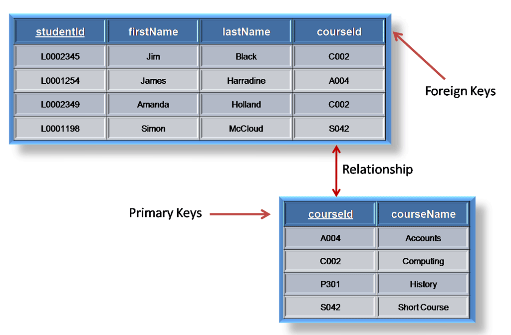
Foreign Keys

The Foreign Key (FK) in an entity is the reference to the primary key of another entity. In the ERD that attribute will be indicated with 'FK' behind its name. The foreign key of an entity can also be part of the primary key, in that case the attribute will be indicated with 'PF' behind its name. This is usually the case with the link-entities, because you usually link two instances only once together (with 1 sale only 1 product type is sold 1 time).

If we put all link-entities, PK's and FK's into the ERD, we get the model as shown below. Please note that the attribute 'products' is no longer necessary in 'Sales', because 'sold products' is now included in the link-table. In the link-table another field was added, 'quantity', that indicates how many products were sold. The quantity field was also added in the stock-table, to indicate how many products are still in store.

Figure 11: Primary keys and foreign keys.

Defining the Attribute's Data Type

Now it is time to figure out which data types need to be used for the attributes. There are a lot of different data types. A few are standardized, but many databases have their own data types that all have their own advantages. Some databases offercthe possibility to define your own data types, in case the standard types cannot do the things you need.

The standard data types that every database knows, and are most-used, are: CHAR, VARCHAR, TEXT, FLOAT, DOUBLE, and INT.

Text:

CHAR(length) - includes text (characters, numbers, punctuations...). CHAR has as characteristic that it always saves a fixed amount of positions. If you define a CHAR(10) you can save up to ten positions maximum, but if you only use two positions the database will still save 10 positions. The remaining eight positions will be filled by spaces.

VARCHAR(length) - includes text (characters, numbers, punctuation...). VARCHAR is the same as CHAR, the difference is that VARCHAR only takes as much space as necessary.

TEXT - can contain large amounts of text. Depending on the type of database this can add up to gigabytes.

Numbers:

·         INT - contains a positive or negative whole number. A lot of databases have variations of the INT, such as TINYINT, SMALLINT, MEDIUMINT, BIGINT, INT2, INT4, INT8.

·         These variations differ from the INT only in the size of the figure that fits into it.

·         A regular INT is 4 bytes (INT4) and fits figures from -2147483647 to +2147483646, or if you define it as UNSIGNED from 0 to 4294967296. The INT8, or BIGINT, can get even bigger in size, from 0 to 18446744073709551616, but takes up to 8 bytes of diskspace, even if there is just a small number in it.

·         FLOAT, DOUBLE - The same idea as INT, but can also store floating point numbers. . Do note that this does not always work perfectly. For instance in MySQL calculating with these floating point numbers is not perfect, (1/3)*3 will result with MySQL's floats in 0.9999999, not 1.

Other types:

BLOB - for binary data such as files. INET - for IP addresses. Also useable for net masks.

For our example the data types are as follows:

Figure 12: Data model displaying data types.

Normalization

Collecting the data from :http://agiledata.org/essays/dataNormalization.html

Data normalization is a process in which data attributes within a data model are organized to increase the cohesion of entity types.  In other words, the goal of data normalization is to reduce and even eliminate data redundancy, an important consideration for application developers because it is incredibly difficult to stores objects in a relational database that maintains the same information in several places.  Table 1 summarizes the three most common forms of normalization ( First normal form (1NF), Second normal form (2NF), and Third normal form (3NF)) describing how to put entity types into a series of increasing levels of normalization. Higher levels of data normalization are beyond the scope of this article.  With respect to terminology, a data schema is considered to be at the level of normalization of its least normalized entity type.  For example, if all of your entity types are at second normal form (2NF) or higher then we say that your data schema is at 2NF. 

Data Normalization Rules :

Level	Rule
First normal form (1NF)	An entity type is in 1NF when it contains no repeating groups of data.
Second normal form (2NF)	An entity type is in 2NF when it is in 1NF and when all of its non-key attributes are fully dependent on its primary key.
Third normal form (3NF)	An entity type is in 3NF when it is in 2NF and when all of its attributes are directly dependent on the primary key.

1. First Normal Form (1NF)

Let’s consider an example. An entity type is in first normal form (1NF) when it contains no repeating groups of data. For example, in Figure 1 you see that there are several repeating attributes in the data Order0NF table – the ordered item information repeats nine times and the contact information is repeated twice, once for shipping information and once for billing information. Although this initial version of orders could work, what happens when an order has more than nine order items?  Do you create additional order records for them?  What about the vast majority of orders that only have one or two items?  Do we really want to waste all that storage space in the database for the empty fields? Likely not.  Furthermore, do you want to write the code required to process the nine copies of item information, even if it is only to marshal it back and forth between the appropriate number of objects.  Once again, likely not. 

Fig1 : An Initial Data Schema for Order (UML Notation) :

 Figure 2 presents a reworked data schema where the order schema is put in first normal form.  The introduction of the OrderItem1NF table enables us to have as many, or as few, order items associated with an order, increasing the flexibility of our schema while reducing storage requirements for small orders (the majority of our business).  The ContactInformation1NF table offers a similar benefit, when an order is shipped and billed to the same person (once again the majority of cases) we could use the same contact information record in the database to reduce data redundancy.  OrderPayment1NF was introduced to enable customers to make several payments against an order - Order0NF could accept up to two payments, the type being something like "MC" and the description "MasterCard Payment", although with the new approach far more than two payments could be supported. Multiple payments are accepted only when the total of an order is large enough that a customer must pay via more than one approach, perhaps paying some by check and some by credit card.

Fig 2 : An Order Data Schema in 1NF (UML notation) :

An important thing to notice is the application of primary and foreign keys in the new solution. Order1NF has kept OrderID, the original key of Order0NF, as its primary key.  To maintain the relationship back to Order1NF, the OrderItem1NF table includes the OrderID column within its schema, which is why it has the stereotype of FK.  When a new table is introduced into a schema, in this case OrderItem1NF, as the result of first normalization efforts it is common to use the primary key of the original table (Order0NF) as part of the primary key of the new table. BecauseOrderID is not unique for order items, you can have several order items on an order, the column ItemSequence was added to form a composite primary key for the OrderItem1NF table. A different approach to keys was taken with the ContactInformation1NF table. The column ContactID, a surrogate key that has no business meaning, was made the primary key. 

Second Normal Form (2NF)

Although the solution presented in Figure 2 is improved over that of Figure 1, it can be normalized further.  Figure 3 presents the data schema of Figure 2 in second normal form (2NF). an entity type is in second normal form (2NF) when it is in 1NF and when every non-key attribute, any attribute that is not part of the primary key, is fully dependent on the primary key. This was definitely not the case with the OrderItem1NF table, therefore we need to introduce the new table Item2NF.  The problem with OrderItem1NF is that item information, such as the name and price of an item, do not depend upon an order for that item. For example, if Hal Jordan orders three widgets and Oliver Queen orders five widgets, the facts that the item is called a “widget" and that the unit price is $19.95 is constant. This information depends on the concept of an item, not the concept of an order for an item, and therefore should not be stored in the order items table – therefore the Item2NF table was introduced. OrderItem2NF retained the TotalPriceExtended column, a calculated value that is the number of items ordered multiplied by the price of the item. The value of the SubtotalBeforeTax column within the Order2NF table is the total of the values of the total price extended for each of its order items.

Fig 3. An Order in 2NF (UML notation) :

Third Normal Form (3NF)

An entity type is in third normal form (3NF) when it is in 2NF and when all of its attributes are directly dependent on the primary key. A better way to word this rule might be that the attributes of an entity type must depend on all portions of the primary key.  In this case there is a problem with the OrderPayment2NF table, the payment type description (such as “Mastercard" or “Check") depends only on the payment type, not on the combination of the order id and the payment type. To resolve this problem the PaymentType3NF table was introduced in Figure 4, containing a description of the payment type as well as a unique identifier for each payment type.

Fig 4. An Order in 3NF (UML notation) :

Beyond 3NF

The data schema of Figure 4 can still be improved upon, at least from the point of view of data redundancy, by removing attributes that can be calculated/derived from other ones.  In this case we could remove the SubtotalBeforeTax column within the Order3NF table and the TotalPriceExtended column of OrderItem3NF, as you see in Figure 5.

Fig 5 . An Order without Calculated Values (UML notation) :

Why Data Normalization?

The advantage of having a highly normalized data schema is that information is stored in one place and one place only, reducing the possibility of inconsistent data. Furthermore, highly-normalized data schemas in general are closer conceptually to object-oriented schemas because the object-oriented goals of promoting high cohesion and loose coupling between classes results in similar solutions (at least from a data point of view). This generally makes it easier to map your objects to your data schema. 

Denormalization

From a purist point of view you want to normalize your data structures as much as possible, but from a practical point of view you will find that you need to 'back out" of some of your normalizations for performance reasons. This is called "denormalization". For example, with the data schema of Figure 1 all the data for a single order is stored in one row (assuming orders of up to nine order items), making it very easy to access.  With the data schema of Figure 1 you could quickly determine the total amount of an order by reading the single row from the Order0NF table.  To do so with the data schema of Figure 5 you would need to read data from a row in the Order table, data from all the rows from the OrderItem table for that order and data from the corresponding rows in the Item table for each order item. For this query, the data schema of Figure 1 very likely provides better performance. 

Glossary

Attributes - detailed data about an entity, such as price, length, name
Cardinality - the relationship between two entities, in figures. For example, a person can place multiple orders.
Entities - abstract data that you save in a database. For example: customers, products.
Foreign key (FK) - a referral to the Primary Key of another table. Foreign Key-columns can only contain values that exist in the Primary Key column that they refer to.
Key - a key is used to point out records. The most well-known key is the Primary Key (see Primary Key).
Normalization - A flexible data model needs to follow certain rules. Applying these rules is called normalizing.
Primary key - one or more columns within a table that together form a unique combination of values by which each record can be pointed out separately. For example: customer numbers, or the serial number of a product.

SELECT: The SELECT statement is used to select data from a database. The result is stored in a result table, called the result-set.

Syntax:

                SELECT column_name(s)FROM table_name

                                                and

                SELECT * FROM table_name

P_Id	Name	Address	City
1	Ram	ameerpet	Hyderabad
2	Robert	s.r.nagar	Hyderabad
3	Raheem	mithrivanam	Hyderabad

Now we want to select the content of the columns named "LastName" and "FirstName" from the table above. 

                SELECT Name FROM Persons

The result-set will look like this:

Name

Ram

Robert

Raheem

Now we want to select all the columns from the "Persons" table.

                SELECT * FROM Persons

Tip: The asterisk (*) is a quick way of selecting all columns!

The result-set will look like this:

P_Id	Name	Address	City
1	Ram	ameerpet	Hyderabad
2	Robert	s.r.nagar	Hyderabad
3	Raheem	mithrivanam	Hyderabad

SELECT DISTINCT

·         In a table, some of the columns may contain duplicate values.

·         This is not a problem; however, sometimes you will want to list only the different (distinct) values in a table.

·         The DISTINCT keyword can be used to return only distinct (different) values.

Syntax

                SELECT DISTINCT column_name(s)FROM table_name

P_Id	LastName	FirstName	Address	City
1	Hansen	Ola	Timoteivn 10	Sandnes
2	Svendson	Tove	Borgvn 23	Sandnes
3	Pettersen	Kari	Storgt 20	Stavanger

Now we want to select only the distinct values from the column named "City" from the table above.

                SELECT DISTINCT City FROM Persons

The result-set will look like this:

City

Sandnes

Stavanger

WHERE Clause

The WHERE clause is used to extract only those records that fulfill a specified criterion.

Syntax

                SELECT column_name(s)FROM table_name WHERE column_name operator value

P_Id	LastName	FirstName	Address	City
1	Hansen	Ola	Timoteivn 10	Sandnes
2	Svendson	Tove	Borgvn 23	Sandnes
3	Pettersen	Kari	Storgt 20	Stavanger

Now we want to select only the persons living in the city "Sandnes" from the table above.

                SELECT * FROM Persons WHERE City='Sandnes'

The result-set will look like this:

P_Id	LastName	FirstName	Address	City
1	Hansen	Ola	Timoteivn 10	Sandnes
2	Svendson	Tove	Borgvn 23	Sandnes

Quotes around Text Fields

SQL uses single quotes around text values (most database systems will also accept double quotes).

However, numeric values should not be enclosed in quotes.

For text values:

                SELECT * FROM Persons WHERE FirstName='Tove'(correct)

                SELECT * FROM Persons WHERE FirstName=Tove(wrong)

For numeric values:

                SELECT * FROM Persons WHERE Year=1965(correct)

                SELECT * FROM Persons WHERE Year='1965'(wrong)

Operators Allowed in the WHERE Clause

Operator	Description
=	Equal
<>	Not equal
>	Greater than
<	Less than
>=	Greater than or equal
<=	Less than or equal
BETWEEN	Between an inclusive range
LIKE	Search for a pattern
IN	To specify multiple possible values for a column

Note:  In some versions of SQL the <> operator may be written as !=

AND & OR Operators

·         The AND operator displays a record if both the first condition and the second condition are true.

·         The OR operator displays a record if either the first condition or the second condition is true.

·         Now we want to select only the persons with the first name equal to "Tove" AND the last name equal to "Svendson":

We use the following SELECT statement:

                SELECT * FROM Persons WHERE FirstName='Tove' AND LastName='Svendson'

P_Id	LastName	FirstName	Address	City
2	Svendson	Tove	Borgvn 23	Sandnes

OR Operator Example

Now we want to select only the persons with the first name equal to "Tove" OR the first name equal to "Ola":

We use the following SELECT statement:

                SELECT * FROM Persons WHERE FirstName='Tove' OR FirstName='Ola'

P_Id	LastName	FirstName	Address	City
1	Hansen	Ola	Timoteivn 10	Sandnes
2	Svendson	Tove	Borgvn 23	Sandnes

Combining AND & OR

You can also combine AND and OR (use parenthesis to form complex expressions).

Now we want to select only the persons with the last name equal to "Svendson" AND the first name equal to "Tove" OR to "Ola":

We use the following SELECT statement:

                SELECT * FROM Persons WHERE LastName='Svendson' AND (FirstName='Tove' OR FirstName='Ola')

P_Id	LastName	FirstName	Address	City
2	Svendson	Tove	Borgvn 23	Sandnes

 

ORDER BY

·         The ORDER BY keyword is used to sort the result-set.

·         The ORDER BY keyword is used to sort the result-set by a specified column.

·         The ORDER BY keyword sorts the records in ascending order by default.

·         If you want to sort the records in a descending order, you can use the DESC keyword.

                SELECT column_name(s)FROM table_name ORDER BY column_name(s) ASC|DESC

P_Id	LastName	FirstName	Address	City
1	Hansen	Ola	Timoteivn 10	Sandnes
2	Svendson	Tove	Borgvn 23	Sandnes
3	Pettersen	Kari	Storgt 20	Stavanger
4	Nilsen	Tom	Vingvn 23	Stavanger

Now we want to select all the persons from the table above, however, we want to sort the persons by their last name.

                SELECT * FROM Persons ORDER BY LastName

P_Id	LastName	FirstName	Address	City
1	Hansen	Ola	Timoteivn 10	Sandnes
4	Nilsen	Tom	Vingvn 23	Stavanger
3	Pettersen	Kari	Storgt 20	Stavanger
2	Svendson	Tove	Borgvn 23	Sandnes

ORDER BY DESC Example

Now we want to select all the persons from the table above, however, we want to sort the persons descending by their last name.

                SELECT * FROM Persons ORDER BY LastName DESC

P_Id	LastName	FirstName	Address	City
2	Svendson	Tove	Borgvn 23	Sandnes
3	Pettersen	Kari	Storgt 20	Stavanger
4	Nilsen	Tom	Vingvn 23	Stavanger
1	Hansen	Ola	Timoteivn 10	Sandnes

 

INSERT INTO: The INSERT INTO statement is used to insert a new row in a table.

·         It is possible to write the INSERT INTO statement in two forms.

·         The first form doesn't specify the column names where the data will be inserted, only their values:

·         INSERT INTO table_name VALUES (value1, value2, value3,...)

·         The second form specifies both the column names and the values to be inserted:

·         INSERT INTO table_name (column1, column2, column3,...) VALUES (value1, value2, value3,...)

SQL INSERT INTO Example

P_Id	LastName	FirstName	Address	City
1	Hansen	Ola	Timoteivn 10	Sandnes
2	Svendson	Tove	Borgvn 23	Sandnes
3	Pettersen	Kari	Storgt 20	Stavanger

Now we want to insert a new row in the "Persons" table.

                INSERT INTO Persons VALUES (4,'Nilsen', 'Johan', 'Bakken 2', 'Stavanger')

P_Id	LastName	FirstName	Address	City
1	Hansen	Ola	Timoteivn 10	Sandnes
2	Svendson	Tove	Borgvn 23	Sandnes
3	Pettersen	Kari	Storgt 20	Stavanger
4	Nilsen	Johan	Bakken 2	Stavanger

Insert Data Only in Specified Columns

It is also possible to only add data in specific columns.

The following SQL statement will add a new row, but only add data in the "P_Id", "LastName" and the "FirstName" columns:

                INSERT INTO Persons (P_Id, LastName, FirstName) VALUES (5, 'Tjessem', 'Jakob')

P_Id	LastName	FirstName	Address	City
1	Hansen	Ola	Timoteivn 10	Sandnes
2	Svendson	Tove	Borgvn 23	Sandnes
3	Pettersen	Kari	Storgt 20	Stavanger
4	Nilsen	Johan	Bakken 2	Stavanger
5	Tjessem	Jakob

UPDATE

The UPDATE statement is used to update existing records in a table.

Syntax

                UPDATE table_name SET column1=value, column2=value2,... WHERE some_column=some_value

Note:  Notice the WHERE clause in the UPDATE syntax. The WHERE clause specifies which record or records that should be updated. If you omit the WHERE clause, all records will be updated!

SQL UPDATE Example

P_Id	LastName	FirstName	Address	City
1	Hansen	Ola	Timoteivn 10	Sandnes
2	Svendson	Tove	Borgvn 23	Sandnes
3	Pettersen	Kari	Storgt 20	Stavanger
4	Nilsen	Johan	Bakken 2	Stavanger
5	Tjessem	Jakob

Now we want to update the person "Tjessem, Jakob" in the "Persons" table.

                UPDATE Persons SET Address='Nissestien 67', City='Sandnes' WHERE LastName='Tjessem' AND FirstName='Jakob'

P_Id	LastName	FirstName	Address	City
1	Hansen	Ola	Timoteivn 10	Sandnes
2	Svendson	Tove	Borgvn 23	Sandnes
3	Pettersen	Kari	Storgt 20	Stavanger
4	Nilsen	Johan	Bakken 2	Stavanger
5	Tjessem	Jakob	Nissestien 67	Sandnes

SQL UPDATE Warning

Be careful when updating records. If we had omitted the WHERE clause in the example above, like this:

                UPDATE Persons SET Address='Nissestien 67', City='Sandnes'

P_Id	LastName	FirstName	Address	City
1	Hansen	Ola	Nissestien 67	Sandnes
2	Svendson	Tove	Nissestien 67	Sandnes
3	Pettersen	Kari	Nissestien 67	Sandnes
4	Nilsen	Johan	Nissestien 67	Sandnes
5	Tjessem	Jakob	Nissestien 67	Sandnes

 

DELETE

·         The DELETE statement is used to delete rows in a table.

·         DELETE FROM table_name WHERE some_column=some_value

Note: Notice the WHERE clause in the DELETE syntax. The WHERE clause specifies which record or records that should be deleted. If you omit the WHERE clause, all records will be deleted!

SQL DELETE Example

P_Id	LastName	FirstName	Address	City
1	Hansen	Ola	Timoteivn 10	Sandnes
2	Svendson	Tove	Borgvn 23	Sandnes
3	Pettersen	Kari	Storgt 20	Stavanger
4	Nilsen	Johan	Bakken 2	Stavanger
5	Tjessem	Jakob	Nissestien 67	Sandnes

Now we want to delete the person "Tjessem, Jakob" in the "Persons" table.

                DELETE FROM Persons WHERE LastName='Tjessem' AND FirstName='Jakob'

P_Id	LastName	FirstName	Address	City
1	Hansen	Ola	Timoteivn 10	Sandnes
2	Svendson	Tove	Borgvn 23	Sandnes
3	Pettersen	Kari	Storgt 20	Stavanger
4	Nilsen	Johan	Bakken 2	Stavanger

Delete All Rows:

It is possible to delete all rows in a table without deleting the table. This means that the table structure, attributes, and indexes will be intact:

DELETE FROM table_name
                or
DELETE * FROM table_name

Note: Be very careful when deleting records. You cannot undo this statement!

CREATE DATABASE

The CREATE DATABASE statement is used to create a database.

Syntax:

                CREATE DATABASE database_name

Example

                CREATE DATABASE my_db

 

CREATE TABLE 

The CREATE TABLE statement is used to create a table in a database.

Syntax

                CREATE TABLE table_name
                (
                column_name1 data_type,
                column_name2 data_type,
                column_name3 data_type,
                ....
                );

Example:

                CREATE TABLE Persons
                (
                P_Id int,
                LastName varchar(255),
                FirstName varchar(255),
                Address varchar(255),
                City varchar(255)
                );

P_Id	LastName	FirstName	Address	City

More ’SELECT’ examples:

To see some of the details:

                SQL> select  empno, ename, sal  from emp;

To see all the records:

                SQL> select * from emp;

To  see only those employees whose salary is above 5000 then you can type the following query with where condition

                SQL>select * from emp where sal > 5000;

To see those employees whose salary is less than 5000 then the query will be

                SQL> select * from emp where sal < 5000;

A SELECT statement that retrieves three columns from each row, sorted in ascending sequence by invoice_total

                SELECT invoice_number, invoice_date, invoice_total
                FROM invoices ORDER BY invoice_total

A SELECT statement that retrieves two columns and a calculated value for a specific invoice

                SELECT invoice_id, invoice_total,
                (credit_total + payment_total) AS total_credits
                FROM invoices
                WHERE invoice_id = 17

A SELECT statement that retrieves all invoices between given dates

                SELECT invoice_number, invoice_date, invoice_total
                FROM invoices
                WHERE invoice_date BETWEEN '01-MAY-2008' AND '31-MAY-2008'
                ORDER BY invoice_date

A SELECT statement that returns an empty result set

                SELECT invoice_number, invoice_date, invoice_total
                FROM invoices
                  WHERE invoice_total > 50000

NOT:

Returns TRUE if the following condition is FALSE. Returns FALSE if it is TRUE. If it is UNKNOWN, it remains UNKNOWN. 

                SELECT *   FROM emp   WHERE NOT   (salary BETWEEN 1000 AND 2000);

Condition	Operation	Example
IN	"Equal to any member of" test.  Equivalent to "= ANY".	SELECT * FROM emp   WHERE deptno IN   (10,20);        SELECT * FROM emp   WHERE deptno IN (SELECT deptno FROM dept WHERE city=’HYD’)
NOT IN	Equivalent to "!=ALL".    Evaluates to FALSEif any member of the set is NULL.	SELECT * FROM emp   WHERE ename NOT IN  ('SCOTT', 'SMITH');

LIKE Conditions

For example you want to see all employees whose name starts with S char. Then you can use LIKE condition as follows

                SQL> select * from emp where ename like ‘S%’ ;

Similarly you want to see all employees whose name ends with “d”

                SQL>select * from emp where ename like ‘%d’;

You want to see all employees whose name starts with ‘A’ and ends with ‘d’ like ‘Abid’, ’Adward’, ’Arnold’.

                SQL>select * from emp where ename like ‘A%d’;

You want to see those employees whose name contains character ‘a’ anywhere in the string.

                SQL> select * from emp where ename like ‘%a%’;

To see those employees whose name contains ‘a’ in second position.

                SQL>select * from emp where ename like ‘_a%’;

To see those employees whose name contains ‘a’ as last second character.

                SQL>select * from emp where ename like ‘%a_’;

To see those employees whose name contain ‘%’ sign.  i.e. ‘%’ sign has to be used as literal not as wild char.

                SQL> select * from emp where ename like ‘%\%%’ escape ‘\’;

EXISTS Conditions:

An EXISTS condition tests for existence of rows in a subquery.

The following example shows the EXISTS condition.

Condition	Operation	Example
EXISTS	TRUE if a subquery returns at least one row.	SELECT deptno   FROM dept d   WHERE EXISTS (SELECT * FROM emp e WHERE d.deptno = e.deptno);

The following is an example of how you might insert 3 rows into the suppliers table in Oracle, using an SQL INSERT statement:

INSERT ALL:

                INTO suppliers (supplier_id, supplier_name) VALUES (1000, 'IBM')

                INTO suppliers (supplier_id, supplier_name) VALUES (2000, 'Microsoft')

                 INTO suppliers (supplier_id, supplier_name) VALUES (3000, 'Google')

                SELECT * FROM dual;

SAMPLE SQL Clause

                Oracle Database provides the SAMPLE clause that can be issued with a SELECT statement over a table. In the following query, we're randomly selecting records from the CUSTOMERS table with a 20% probability. 
                  SELECT * FROM customers SAMPLE (20);

This means that each record has a 20% chance of being selected. Perhaps contrary to expectations, this will normally not produce a result with 20% of the records from the CUSTOMERS table. This approximate sample size is quite adequate for most situations. 

Sql>SELECT COUNT(*) FROM t;

Sql>SELECT COUNT(*) * 0.1 FROM t;

Sql>SELECT * FROM t SAMPLE(1);

Sql>SELECT * FROM t SAMPLE(1);

Sql>SELECT * FROM t SAMPLE(1);

Sql> SELECT * FROM t SAMPLE(35) WHERE object_name LIKE '%J%';